Previously, I wrote about how to use Valgrind for debugging memory issues – and today, I’d like to go into how to use the tool for profiling.
As I wrote before, Valgrind is an instrumentation framework that provides a collection of tools. For profiling, we’ll look at the Callgrind tool together a GUI application called KCachegrind. As a quick historical note, the predecessor to Callgrind is called Cachegrind, and was mostly for examining CPU cache usage – but Callgrind was developed out of that. KCachegrind, on the other hand, kept the old name.
Example Code #1
Let’s again start with some example code.
#include <cstdint>
#include <string>
#include <map>

struct foo
{
  int bar;
};

template <typename mapT>
void
do_stuff(mapT & map, int amount)
{
  for (int i = 0 ; i < amount ; ++i) {
    map[std::to_string(i)] = foo{i};
  }
}


int main(int argc, char **argv)
{
  std::map<std::string, foo> map;
  do_stuff(map, 1_000_000);
}
It is as simple as it can get. The main point is to demonstrate a relatively work intensive loop. In this case, we have a function that adds an amount of objects to a map, where the key to the map is a string. It just so happens to be the value of the counter we’re using, but that is just for generating strings easily.
We’ve made this a function template because it means we’ll keep the loop code exactly the same throughout the rest of this post.
Our example here requests one million objects, just to do some real work.
As before, there is no particular way this needs to be compiled, but it becomes
clearer when smaller functions aren’t automatically inlined. So on Linux (gdb or
clang), I pass -O0 to optimize nothing.
Analysis with Callgrind #1
This time around we’re passing a different tool to Valgrind. We’ll also ask it to output to a log file, because the console is less helpful here.
$ valgrind --tool=callgrind --callgrind-out-file=map.log \
      ./example
You’ll find that running the example with and without Valgrind/Callgrind makes a significant difference in execution speed. This is because Callgrind counts a few things when running the code, including how often each function gets invoked.
We then run KCachegrind over the resulting log:
$ kcachegrind map.log
This produces the following view (you might want to click on it to open a larger version):
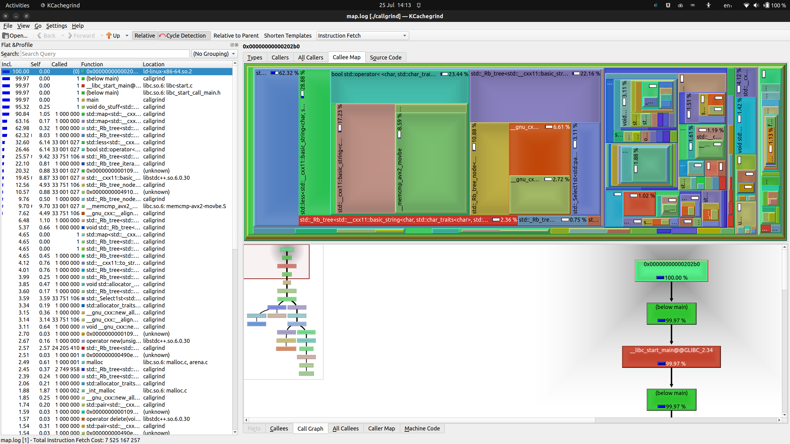
Figure: KCachegrind showing map.log
The main view is subdivided into three panels:
-
On the left, there is a flat list of functions, ordered by cumulative cost. Other than some bootstrapping functions, it should come as no surprise that
main()is at the top of the list. In theCalledcolumn, you can see it was called exactly once. Also, our owndo_stuff()was called once, as is to be expected.The percentages in the “Incl.” and “Self” columns are the cost. The first of these lists the cost of the function including all of the costs of all of the functions it calls, while the second lists how much function’s own code costs (I’ll get back to that later).
-
The top panel is dominated by a colourful “Callee Map”. This is a map visualization of the above two columns. For each function, the relative cumulative cost determines the size of the rectangle it occupies in the map. The blank area is its own cost, while the rectangles nested within it represent the costs of the functions it calls.
The visualization lets you zero in very fast on where in your program time is spent: the larger the blank space, the better the candidate (as a rough rule of thumb).
-
Finally, in the bottom panel, there is a call graph with its own mini map. You can click any of the functions in the call graph to highlight it in the above Callee Map, which helps with navigation.
You may also see that both the top and bottom panel contain multiple tabs. These are effectively different visualizations of the same data, and may prove useful under certain circumstances. KCachegrind defaults to the described tabs because they’re likely the most useful – in my experience, I rarely switch to different views here.
You’ll see that the process listed in the KCachegrind view is called
callgrind. I cheated a little there. I called the programcallgrindwhen running the tests, but called itexampleabove. Sorry.
On Costs
I’ve tried to avoid speaking about how the function cost above is measured, so we can go into it now. If you look above the top panel, you’ll see a drop-down menu which by default has “Instruction Fetch” selected.
Callgrind counts the number of instructions fetched in your program as a proxy for function cost. This is not an exact measure – some individual instructions can take more cycles to execute than others. But the number of instructions in a function is nonetheless a reasonable proxy for how long it may take to execute.
What Callgrind does not do is measure time spent. Wall time in particular depends not only on the software itself, but on how many time slices the kernel allocates for it. On a busy system, a function might execute a lot more slowly than on an idle system. By using instruction fetches, Callgrind becomes independent of current system load in its cost calculation.
That being said, you can select other cost calculations in the drop-down.
Analysis
A quick analysis is possible by looking at the Callee Map. It’s pretty clear that the most cost is in the “left” two thirds of the program, so lets drill down a little.
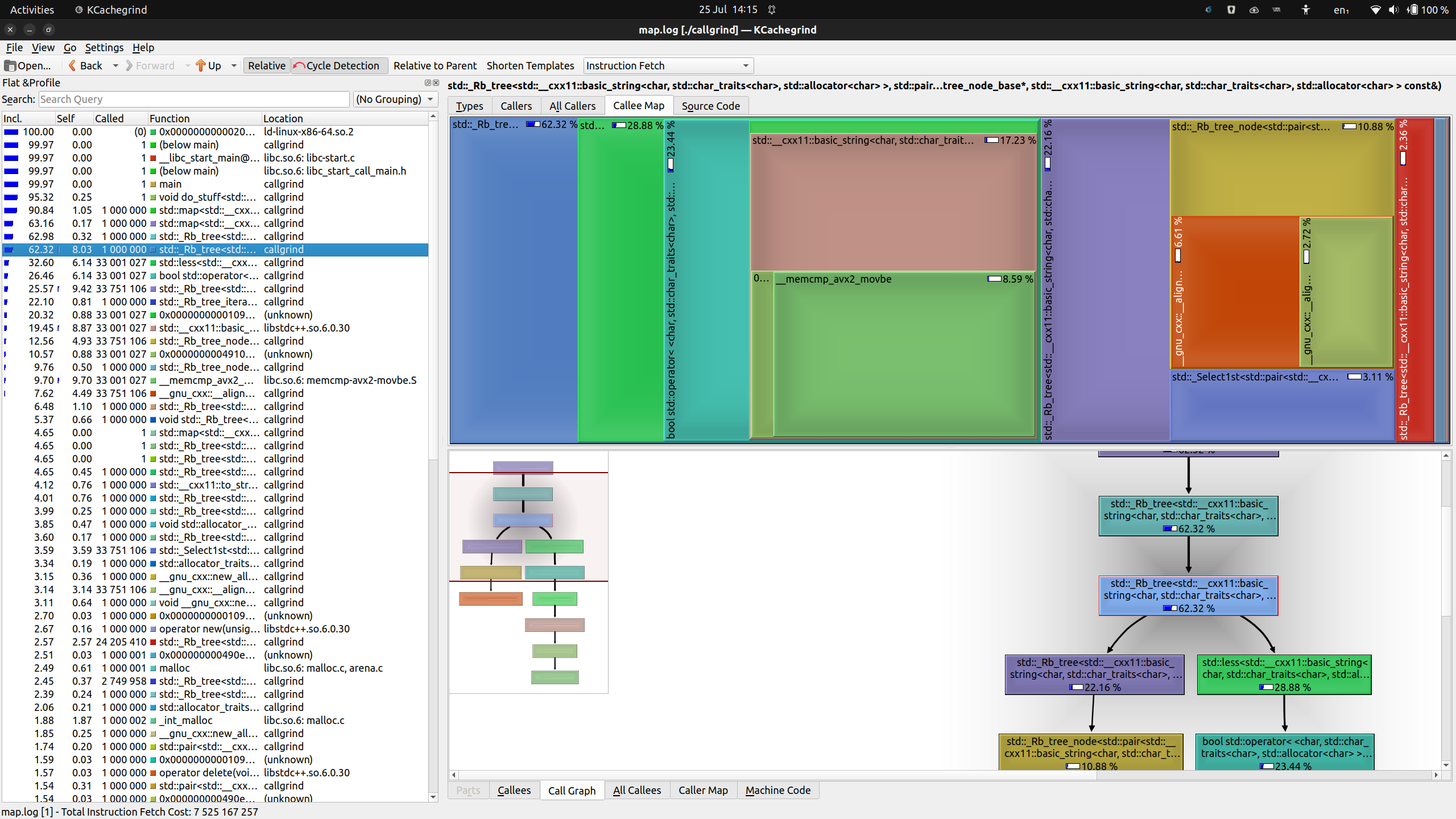
Figure: KCachegrind showing map.log focused on std::less
Drilling down only a little, you can see that the main cost is spent in two
branches: an internal map function that does something with a red-black tree,
which is how map internally keeps elements ordered. And on the other hand, it
spends a lot of time in std::less<std::string>().
None of this should come as a surprise. Maps are ordered, and rebalancing the three has to happen a lot when inserting elements. And to find the order of keys, they will have to be less-than-compared. In our example, keys are strings.
A glance at the left panel shows the RB-tree operation highlighted, which
is called one million times – so once per element inserted. But we can also
see that std::less() is invoked 33 million times – an average of 33 times
per insertion.
It’s also visible that std::less() eventually leads to some optimized
memcmp() function – fair game for string comparison.
So how can we improve this code a little?
Example Code #2
The simplest thing we can do, and which we will do, is replace our ordered
std::map with an unordered std::unordered_map – that should get rid of
all those comparisons, right? Or at least some of them.
#include <map>
#include <unordered_map>

// ...

int main(int argc, char **argv)
{
//  std::map<std::string, foo> map;
  std::unordered_map<std::string, foo> map;
  do_stuff(map, 1_000_000);
}
Quick and painless. And as I mentioned above, the logic of our do_stuff()
function isn’t touched.
Analysis with Callgrind #2
The next run provides a very different picture.
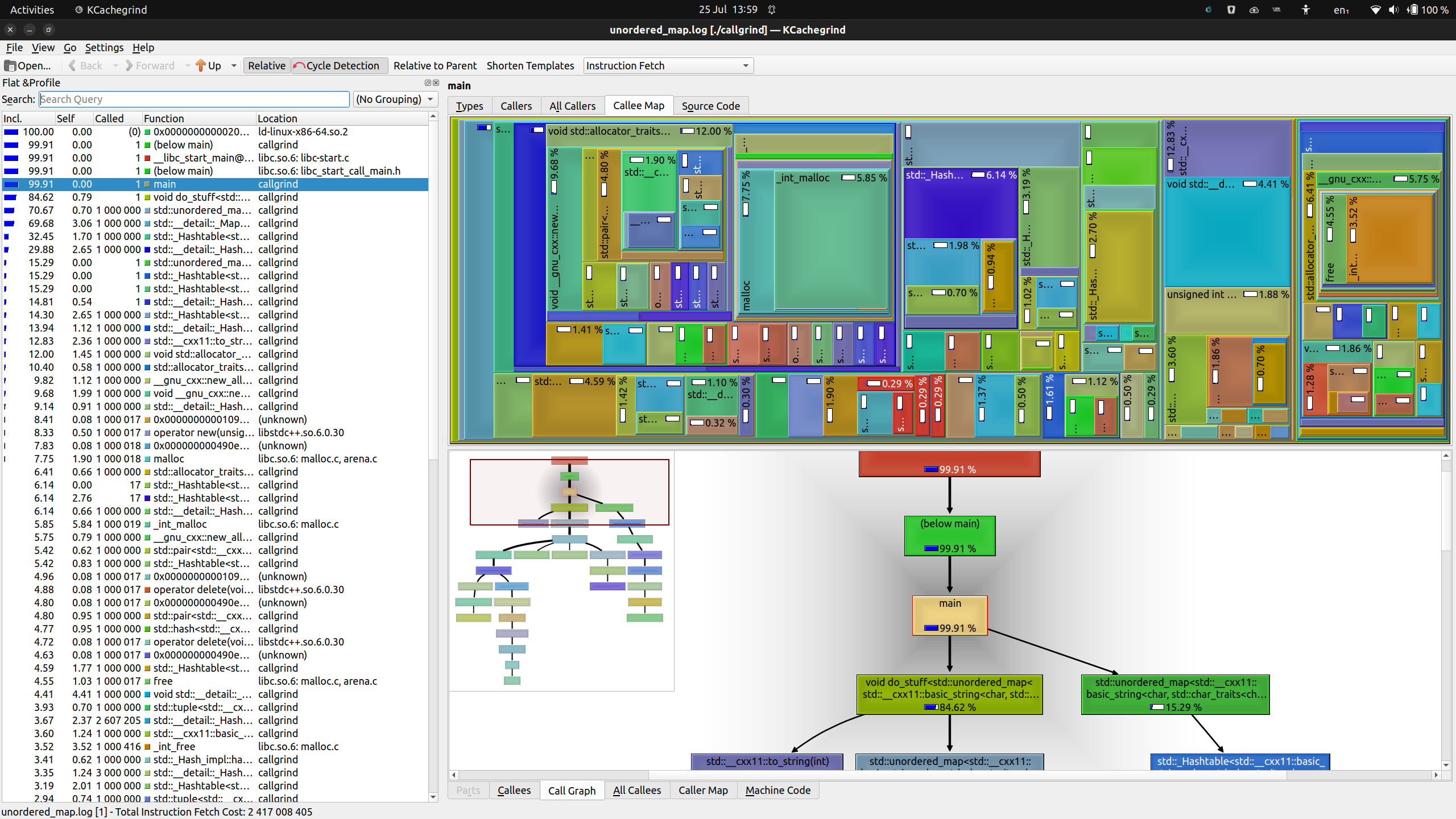
Figure: KCachegrind showing unordered_map.log
Where before, there the “left two thirds” of the call costs clearly dominated, here the picture is a lot more varied. That is generally a good thing for performance. It means that no single function is an outlier in its cost.
The downside, of course, is that things become harder to optimize when there are no outliers.
In the left panel, we can see that each function is called around one million times, so once per insertion. We could shave off instructions in all of those functions.
The only thing that stands out here is that something related to hashing is called up to three million times. Just because this function is called more often, it may make sense to find an optimization here.
If you know anything about the implementation of std::unordered_map, you know
that it’s hash bucket based. A hash of the key is taken, but the hash function
produces collisions, so several keys will match the same hash. This then
creates buckets of keys, which are (typically) added to a list. Within this
list, the map implementation still needs to perform string comparisons, but
those are so few, relatively speaking, that they don’t turn up very high in
the cost list.
That said, the next optimization might involve not having to create hashes of the string keys so often. In our example, that’s easily avoided, but real code may not have that luxury.
However, even though the relative cost of functions to each other is much better balanced, is the actual cost of running the software higher or lower than with the ordered map? Also hashing a string involves some effort, after all.
Analysis with Callgrind #3
One feature of Callgrind may help here, which KCachegrind visualises just fine. You may see a check button at the top that is labelled “Relative”.
What happens when we uncheck it?
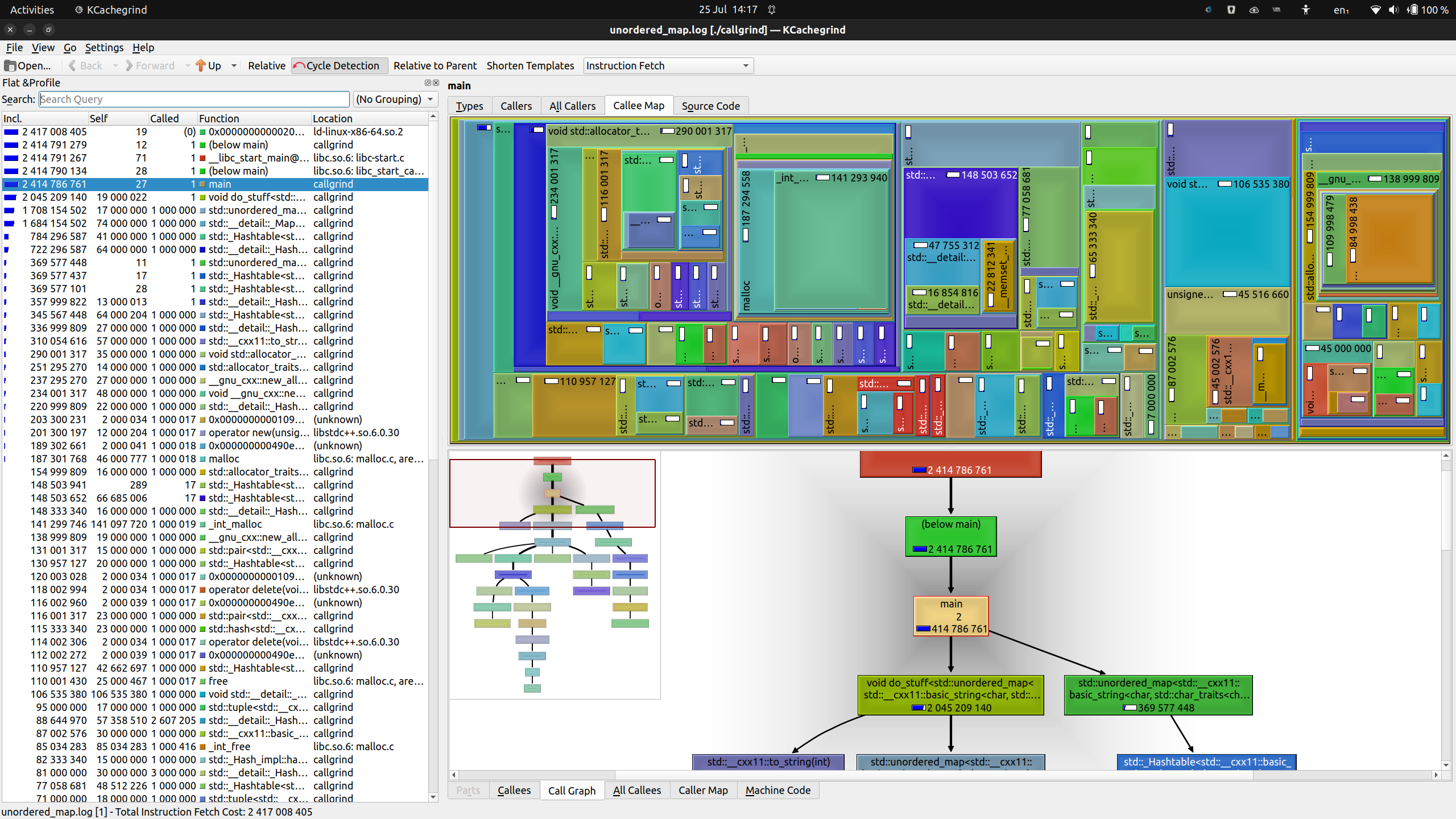
Figure: KCachegrind showing unordered_map.log with absolute costs
You can see that the numbers displayed in both the “Incl.” and “Self” columns on the left, in the Callee Map, as well as in the Call Graph are no longer percentages, but rather large numbers. This is the actual instruction fetch count.
Now we can see that code fetches (and executes) round about 2.4 billion
instructions. Let’s compare this to our regular std::map:
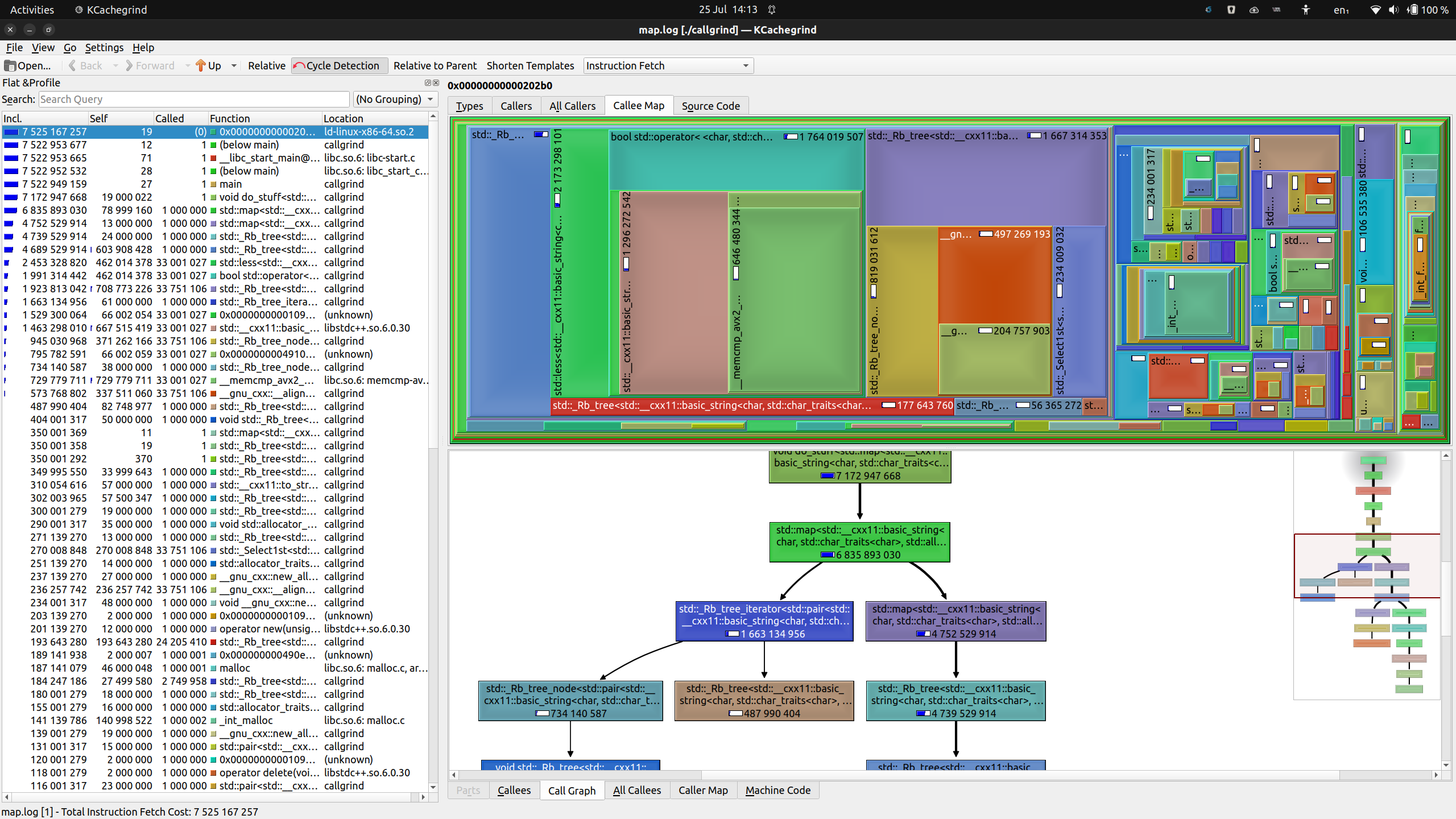
Figure: KCachegrind showing map.log with absolute costs
So, using a regular, ordered map cost around 7.5 billion instructions by comparison. Again, with the caveat that instruction fetches are just a proxy for CPU cycles spent, it seems we cut our overall running cost down to a third.
I’d call that a successful optimization with the help of Callgrind!
Summary
One panel I have not shown here is the “All Callers” tab in the top panel. Sometimes an easy optimization is to look at where a function is called from, and eliminate some of those sites.
The example here is particularly simple – I’m just making choices between some standard library features; there is no optimization I’m performing that is tweaking lovingly handcrafted assembly here.
But that’s also the point I’d like to make here. We’ve all heard that “premature optimization is the root of all evil.” This quote by Sir Tony Hoare (popularized by Donald Knuth), can also be applied more practically.
Before you start breaking out your assembly knowledge and producing a more optimized version of some function, it’s worth just looking at where effort is spent. Sometimes, re-arranging the deck chairs (aka data model) is all that’s needed to make a difference.
And if that’s not good enough, who am I to stop you from assembly programming?